Test
线性可分与凸壳
描述
题目出自《统计学习方法》 P36:设集合$S\subset R^n$ 是由$R^n$中的$k$个点所组成的集合,即$S=\{x_1,x_2,\cdots,x_k\}$,定义$S$的凸壳$conv(S)$为:
证明以下定理:样本集线性可分的充分必要条件是正实例点集所构成的凸壳与负实例点集所构成的凸壳互不相交。
上网查了一遍,只找到半份比较好的证明:http://blog.csdn.net/y954877035/article/details/52210734 对充分性证明起了很大作用(其实是本菜鸡整理补充了一下他的证明过程)。
必要性
必要性: 若样本集线性可分,则正实例点集所构成的凸壳与负实例点集所构成的凸壳互不相交。
采用反证法,假设超平面$f(\hat{x})=\hat{w}\cdot\hat{x}$能完全分开正负样本,即$f(x_+)>0$,$f(x_-)<0$。
假设正类凸壳和负类凸壳相交部分样本点为$z$ ,有定义可知:
其中$ \sum_{i=1}^k\lambda_i=1,\lambda_i\ge0,i=1,2,\cdots,k_1 $
即样本$z$分别可由正样本和负样本按线性加权表示。现考虑$f(z)$:
同理可得,$f(z)<0$,矛盾,故必要性得证。
充分性
(该部分主要来源于http://blog.csdn.net/y954877035/article/details/52210734 特别感谢该CSDN博主!)
再证充分性:若正实例点集所构成的凸壳与负实例点集所构成的凸壳互不相交,则样本集线性可分。
从距离入手。定义两点间的距离为 $dist(x_1,x_2)=\sqrt{(x_1-x_2)\cdot(x_1-x_2)}=\Vert x_1-x_2\Vert _2$ ,也就是二范数。
定义凸壳间的距离为$dist(conv(S_+),conv(S_-))=min\{dist(x_+,x_-) \quad \big| \quad x_+\in conv(S_+),x_-\in conv(S_-) \}$ ,也就是两个凸壳上最接近的点之间的距离。下文记该点对为$x_{+0}$ 和$x_{-0}$ 。
那么显然:对任意$x_+\in conv(S_+),x_-\in conv(S_-)$ , $dist(x_+,x_-)\ge dist(conv(S_+),conv(S_-))=dist(x_{+0},x_{-0}) \tag{3.1}$
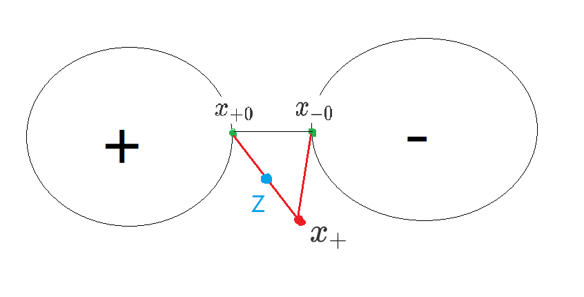
引理1:$dist(x_+,x_{-0})>dist(x_+,x_{+0})$ ,即正类凸壳上的任意点到负类凸壳的距离一定比该点到$x_{+0}$ 的距离大。
其实很显然。想象成过河的情景,你到对面岸的距离显然比你到自己这个岸边的距离要更远。然而证明起来还有点 非常费劲。。
反证法,假设$dist(x_+,x_{-0}) \le dist(x_+,x_{+0})$ ,又有式(2): $dist(x_+,x_{-0})d \ge dist(x_{+0},x_{-0})$ .
即$dist(x_{+0},x_{-0}) \le dist(x_+,x_{-0}) \le dist(x_+,x_{+0}) \tag{3.2}$
取
由式(3.2)可知$t<1$ 。$\theta$="" 表示向量$\overrightarrow{="" x_{+0}="" x_{-0}}$="" 与向量$\overrightarrow{="" x_{+}}$="" 间的夹角。$\theta$="" 所对的边是$\overline{x_+x_{-0}}$="" ,由式(3.2)可知该边为最短的边,故$\theta$="" 小于$90^\circ$="" ,="" 故$t="">0$ 。
取 $z=tx_++(1-t)x_{+0}$ ,故点$z\in conv(S_+)$ 且在线段$\overline{x_{+0} x_+}$ 上。显然$dist(z,x_{-0})<dist(x_{+0},x_{-0})$ ,这与式(3.1)矛盾,引理得证。
下面开始正式证明。直接以线段$\overline{x_{+0}+x_{-0}}$ 的中垂超平面作为判决函数:
考虑对任意正样本$x_+$:
同理,对任意负样本有$w\cdot x_-+b <0$ ,该数据集线性可分。
其实有个凸集分离定理知 直接就证完了,有兴趣的同学可以自行了解。。
感知器学习笔记
最近杨老师课上又学了一遍感知器。。唔,算做个总结吧。 时间仓促,难免有疏漏,望各位指正!(email: vast2stars@gmail.com)
基本
感知器函数定义:
其中$w$ 和$b$ 为感知器模型参数,分别为权值和阈值。在特征空间$R^n$ 中,$w$ 是感知器决策超平面的法向量(恒指向正类$^{[1]}$),$b$ 是超平面的截距。$f(x)$ 输出$+1,-1$ 。
记感知器学习策略的损失函数为$L(w,b)$。 该函数不能定义成误分类点的数量,因为此时$L$ 不是关于$w,b$ 的连续可到函数$^{[2]}$,不易优化。通常采用所有误分类点(集合M)到超平面的距离总和作为损失函数。推导过程如下:
任意点到超平面的距离为:
消除误分类点的符号差异性: 式(1)分子含有绝对值,不利于求微分进行优化。如果删去绝对值,那么假阴性(false negative, FN)样本的计算值为负,而假阳性(false positive, FP)为正,错误相互抵消而非累加。为了解决该问题,使用$-y_i(w\cdot x_i+b)/||w||$ 作为修正后的距离(不论FN还是FP,该函数值恒为正)。
删去$1/||w||$ $^{[3]}$ 并累积求和,得到最终的损失函数:
对上式求微分,即可得到感知器的训练规则。此处略过。
三个不等式
记$\hat{w}=(w^T,b)^T$,$\hat{x}=(x^T,1)^T$,显然$\hat{w}\cdot \hat{x}=w\cdot x+b$。若训练数据集线性可分,则存在超平面可将数据集完全分开,取此超平面为$\hat{w_{opt}}\cdot \hat{x}=0$,且不妨令$||\hat{w}_{opt}||=1$.
取 $\gamma=min_i\{y_i(w_{opt}\cdot x_i+b_{opt})\}$ 。其实$\gamma$ 就是误分类样本点到超平面距离的最小值。
记$\hat{w}_k$是第$k$次迭代后的参数,学习过程:
$||\hat{w}_k||$上界
由三角不等式及式(2.1),有:$||\hat{w}_k||\le||\hat{w}_{k-1}||+||\eta y_k\hat{x}_k||=||\hat{w}_{k-1}||+\eta ||y_k||\cdot||\hat{x}_k||$
考虑到$y_k$ 符号不确定,我们平方处理:
考虑$y_k\hat{w}_{k-1}\cdot \hat{x}_k$, 由于第$k$个样本$\hat{x}_k$相对于参数$\hat{w}_{k-1}$是错误的,则$\hat{w}_{k-1}\cdot \hat{x}_k$ 一定与$y_k$异号(见上文消除误分类点的符号差异性 ),故$y_k\hat{w}_{k-1}\cdot \hat{x}_k\le0$。
所以我们有:
$||\hat{w}_k||$下界
所以就$\hat{w}_k\ge\frac {k\eta\gamma} {\hat{w}_{opt}}$ ?大错特错。2个向量之间不能比较大小。况且点乘【 $\cdot$ 】 不是实数的乘法。
考虑$k\eta\gamma\le\hat{w}_k\cdot\hat{w}_{opt}\le||\hat{w}_k||\times||\hat{w}_{opt}||$ ,所以我们有:
$k$上界
结合(2.2)和(2.3),且$||\hat{w}_{opt}||=1$,我们有:
即$k^2\gamma^2\le kR^2$ ,得:
变形
假设感知器的函数输出函数sign() 以及样本类标$y_i$类标为0和+1,那么如何进行以上证明?
首先考虑到以上所有推导证明都不涉及感知器的输出函数sign ,而公式里大多都和$y_i$ 有关。下面从$y_i$ 角度考虑。
同样,到超平面的距离仍然是式(1)。但是在消除误分类点的符号差异性时,有两种方法:
- 取$y^{new}_i=2\times (y_i-0.5)$, 这样就把$\{0,+1\}$ 映射到$\{-1,+1\}$ ,所有后面的证明都相同。
- 上课说的,取 $y^{new}_i=y_i-\hat{w}\cdot\hat{x} $, 若是FP,$\hat{w}\cdot\hat{x}>0$ , $y_i^{new}<0$ ;="" 若是fn,="" 同理$y_i^{new}="">0$ 映射到$(-\infty,0)\cup(0,\infty)$ 。当然这个变换缺陷是关于FP和FN是不对称的,且输出值不是固定值,不如方法1方便。优点是对所有样本都可以进行该变换,如果是分类正确的样本,$y_i^{new}=0$ ,在计算$L(w,b)$ 时就可以直接对全体样本代入计算,不用判断是否为误分类样本。
补充证明
1 法向量恒指向正样本
证明: 假设$x_0$ 恰好位于决策超平面上,即$w\cdot x_0+b=0$ ,那么从该点引出法向量指向$x_1$,即$x_1=x_0+\alpha w$ 。不失一般性,设$\alpha=1$ 。那么
2 不连续
在$L$ 定义成误分类点的个数时,$L$ 很难(几乎不可能?)写成关于$w,b$ 的解析形式。就算有,那么也是包含数量巨大的脉冲函数(难以求微分)。在这种情况下要求得极小值,相当于一个超高维且分布规律弱的离散优化问题。
3 不考虑$||w||$
显然$w$ 和$b$ 同时按比例放大缩小时,对决策超平面没有任何影响,而感知器学习目标是改进决策超平面的位置。且分子分母同时带有$w$ 不易于函数优化(尤其分母还是欧氏距离函数)。
4 额外证明
题目出自《统计学习方法》 P36:设集合$S\subset R^n$ 是由$R^n$中的$k$个点所组成的集合,即$S=\{x_1,x_2,\cdots,x_k\}$,定义$S$的凸壳$conv(S)$为:
证明以下定理:样本集线性可分的充分必要条件是正实例点集所构成的凸壳与负实例点集所构成的凸壳互不相交。
证明过程见:https://vast-stars.com/2018/03/18/线性可分与凸壳/
参考
[1] 李航. 统计学习方法[M]. 清华大学出版社, 2012.
[2] 杨老师的PPT
[3] http://blog.csdn.net/y954877035/article/details/52210734
浅谈Cost Function
杂谈 Cost Function
cost function 又称为代价函数,又记为loss。本文选取了一些有意思例子来介绍。
先看看我们学过课程中的:
最优化: 调整 $w$ 拟合f(x) loss=均方误差
模式识别: 分类器,以SVM为例,loss= 经验误差 - 几何边缘区 (即在经验误差最小的基础上,尽可能增大分类间隔。减法只是便于理解的一种记号)
人工智能概论: A*算法中的 f=h+g;
1 遗传算法:
1.1 画图

Win下编译好的文件 见这里, 需要windows .net framework 4.0 环境。360等杀毒软件可能会拦截。
可以在 遗传算法图片特效 在线使用。
loss应该定义成画的图和原图的差距。差距越小则loss函数越小,遗传算法可以通过收敛到最优解来使图形越来越准确。
原理说明见:http://songshuhui.net/archives/10462
1.2 解TSP(旅行商问题)
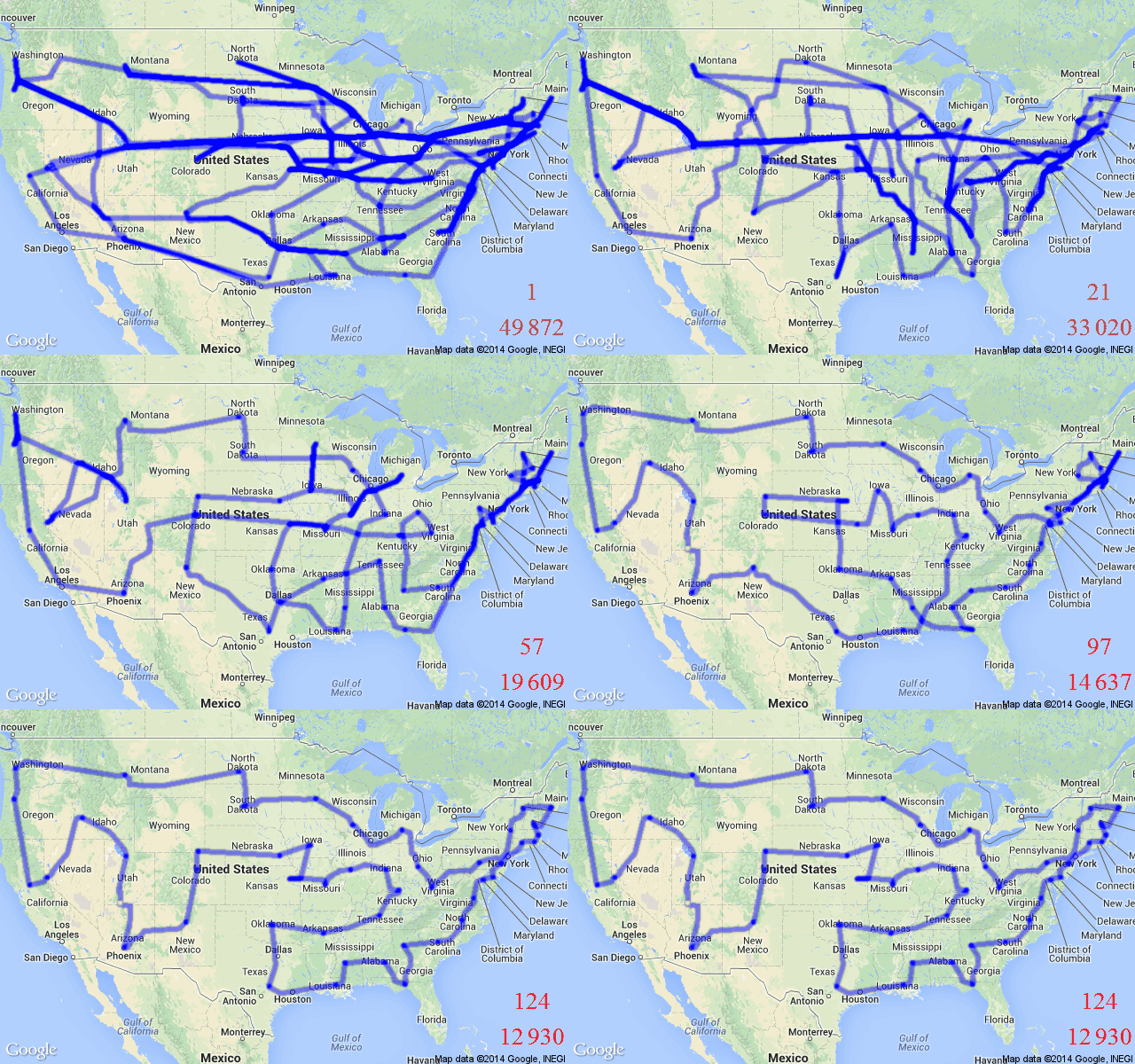
loss=路径总长度。越短越好。
2 蚁群算法:
http://video.tudou.com/v/XMTc4NjQzMDAxNg==.html
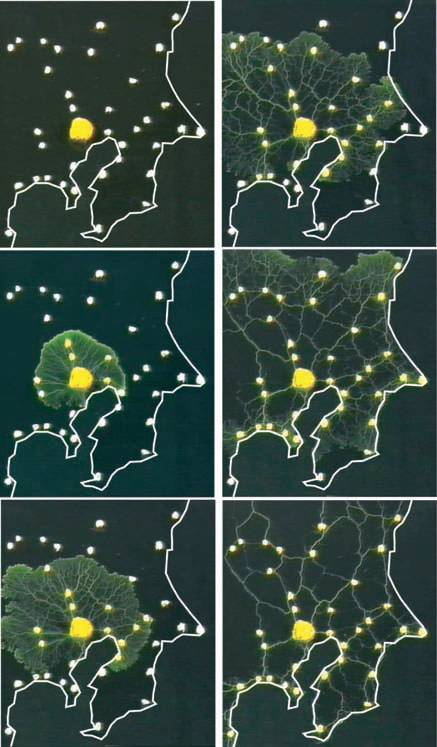
实验很简单,用黏菌避光的特性,用光斑模拟海岸线和地形,在东京附近重要的地铁站对应的位置放上食物:
这是只有海岸线的时候,黏菌铺张、求出最省连通路径的过程图:
下面是用光的强度模拟水域和地势的结果,灰度越高代表光强度越弱(海拔在海平面以上同时越低)。
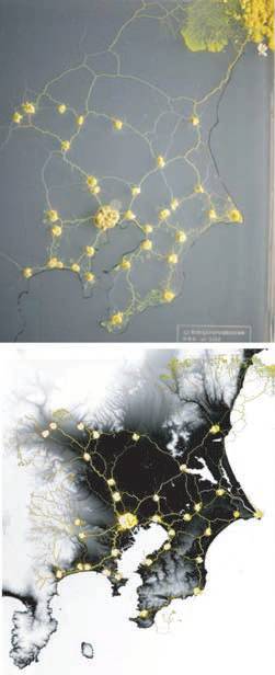
专业的建模分析就不赘述了,科学家最后的原理是黏菌形成的微网络当中,“远路”携带的营养运送过程中消耗大,因而流速低,直径逐渐收缩;而“捷径”流速更大,直径逐渐增大。这样,整个网格就逐渐收缩到最优解上。实际上是一种类似于蚁群算法的退火算法。
实验者模拟了一下这个算法,解出来的结果和黏菌搜索的结果相差无几:
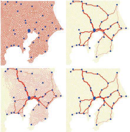
loss≈总能量/总食物 即运输单位“食物”所耗费的能量(即通道长度)。
3深度学习相关:
大家可以自己想想以下项目的loss该怎么设置才能达到预期效果。
http://seeleit.com/songci RNN 宋词生成器
https://www.twitch.tv/sentdex AI GTA5主播
http://www.cs.toronto.edu/~graves/handwriting.cgi?text=i+am+luoyi.+i+am+excited+today.&style=..%2Fdata%2Ftrainset_diff_no_start_all_labels.nc%2C1082%2B554&bias=0.05&samples=3 手写体模仿阿里鲁班:2017年双11将有4亿张人工智能海报由机器人设计。

Cycle GAN 内容很多,科研+工程的典范。
里面有个直播换脸的视频可能无法访问 ,可以见https://weibo.com/1402400261/FpdgrlxoY?type=comment。
Reference
https://rogerjohansson.blog/2008/12/07/genetic-programming-evolution-of-mona-lisa/
维基百科A*算法的错误
先放中文wiki的代码,时间为2017年11月18日16:08:08。
|
|
基友猴哥告诉我,wiki上拓展子节点的时候,如果子节点出现在Close表中话,不做任何处理。而教材人工智能及其应用、算法艺术与信息学竞赛 中均对子节点的F值进行了计算,如果小于表中已有的,则必须更新(加入)到Open表中。而wiki上不论中英文版本均不做处理。那么有什么影响?
抽象的想,从起点S开始有p1、p2两条路径均可到达中间某节点A。假设从p1到达A之后,拓展A的子节点,此时A已加入到S表中,且A的子节点是在A的基础上计算的G值。那么如果路径p2到达A的代价值(G)比p1小,按照wiki的流程图,最终结果还是采用p1这条代价更大的走法,从而无法收敛到最优解(从p2到A)。
多说无益,下面我构造了个例子:
graph LR;
S{S 20}--12-->A{A 13};
S--10-->B{B 16};
B--1-->A;
A--15-->D{D 10};
起点是S,目标是X(未画出,在D之后)。节点内部的数字表示H估值,变上面的数字代表G代价。以下是按照wiki的流程:
格式为:A(G,H) 粗体表示最小F值节点。 斜体表示新加入节点。
| Step | Open | Close |
|---|---|---|
| 1 | A(12,13) B(10,16) | null |
| 2 | B(10,18) D(12+15,10) | A(12,13) |
| 3 | D(12+15,10) | A(12,13) |
到这里,拓展B的时候发现A已经在Close表中,就不采取任何操作,而D(F=37)和D之后节点的G值都是在A 12的基础上计算,明显比S→B→A(只需要11)大,故在这种情况下得到的不是最优解。
而采用更像放回Open表中的情况呢?
| Step | Open | Close |
|---|---|---|
| 1 | A(12,13) B(10,16) | null |
| 2 | B(10,18) D(12+15,10) | A(12,13) |
| 3 | D(12+5,10) A(10+1,13) | B(10,18) |
| 4 | D(10+1+15,10) | B(10,18) A(10+1,13) |
此时D的F值为26+10=36,路径是S→B→A→D,是最优路径。
A* Algorithm and 8 Puzzle Problem
一 A* 算法
1.1 算法介绍
1.1.1 相关背景
广度优先搜索(Breadth-First-Search,BFS)、深度优先搜索(Depth-First-Search,DFS)以及由此延伸出来的双向广度优先搜索(DBFS)、双向深度优先搜索(DDFS)都属于盲目搜索,这在状态空间不大的情况下是很合适的算法,可是当状态空间十分庞大时,它们的效率实在太低,往往都是在搜索了大量无关的状态结点后才碰到解答,甚至更本不能碰到解答。搜索是一种试探性的查寻过程,为了减少搜索的盲目性引,增加试探的准确性,就要采用启发式搜索了。所谓启发式搜索就是在搜索中要对每一个搜索的位置进行评估,从中选择最好、可能容易到达目标的位置,再从这个位置向前进行搜索,这样就可以在搜索中省略大量无关的结点,提高了速度。
1.1.2 A*算法流程
A*算法是一种启发式搜索算法,可以看做是针对盲目搜索(BFS/DFS)的优化。相对于DFS,A*仅仅多了一个评估值H,使状态空间不那么盲目。在A*算法中,一个结点位置的好坏用估价函数(H)来对它进行评估。A*算法的估价函数可表示为:
其中,$F’(n)$ 是估价函数,$g’(n)$ 是从初始起点到当前节点$n$的最短路径值(也称为最小耗费或最小代价,在盲目搜索中对应搜索深度), $h’(n)$ 是当前节点$n$ 到目标节点的最短路径的启发值。由于这个$f’(n)$ 其实是无法预先知道的,所以实际上使用的是下面的估价函数:
其中$g(n)$ 是从初始结点到当前节点n的实际代价,$h(n)$ 是从当前结点n到目标结点的最佳路径的估计代价。在这里主要是$h(n)$ 体现了搜索的启发信息,因为$g(n)$ 是已知的。用$f(n)$ 作为$f’(n)$ 的近似,也就是用$g(n)$ 代替$g’(n)$ 、$h(n)$ 代替$h’(n)$ , 这样必须满足以下条件:
- $g(n)\ge g’(n)$ . 大多数情况下都是满足的,可以不用考虑。 $g(n)$ 必须保持单调递增。
- $h(n)$ 必须小于等于实际的从当前节点n到达目标节点的最小耗费,即$h(n)\le h’(n)$ , 可以证明应用这样的估价函数是可以找到最短路径的。
A*算法基本上与BFS相同。区别在于扩展出一个结点后,要计算它的估价函数(f),并根据估价函数对待扩展的结点排序,从而保证每次扩展的结点都是估价函数(f)最小的结点。
具体步骤:
- 新建一个
Open和Closed表,置空,将初始状态放入Open表中。 - 将
Open表中最小F值状态取出放入Closed表中,若找到目标状态,则中断过程,此时状态的GG值就是最短路径(在八数码是最少步骤),否则生成其下一步所有能转移的状态集S - 计算状态集S每个状态的F,G,H值,得出F=G+H值,这里的G可取前一个状态(父状态)的GG值加一,为了寻得最短路径,可将其指向父状态。
- 枚举状态集,按5, 6处理
- 若状态集S的状态在
Closed表中,则不理会,否则6 - 若状态集S的状态在
Open表中且其F值较小,则更新(因为有最优的路径啊当然要更新),否则不理会,若不在Open表中,则插入。 - 进入2
伪代码:(源自wiki) 有错误 见我的博客
|
|
1.1.3 其他
- 如果$g(n)$ 为0,即只计算任意顶点$n$ 到目标的评估函数$h(n)$ ,而不计算起点到顶点$n$ 的距离,则算法转化为使用贪心策略的Best-First Search,速度最快,但可能得不出最优解;
- 如果$h(n)$ 不高于实际到目标顶点的距离,则一定可以求出最优解,而且$h(n)$ 越小,需要计算的节点越多,算法效率越低,常见的评估函数有——欧几里得距离、曼哈顿距离、切比雪夫距离;
- 如果$h(n)$ 为0,即只需求出起点到任意顶点$n$的最短路径 ,而不计算任何评估函数$h(n)$ ,则转化为单源最短路径问题,即Dijkstra算法,此时需要计算最多的定点;
1.2 C++实现
1.2.1 数据结构
A*算法主要数据结构为Open表和Close表。其中,Open 表有取最小值、查找、插入、删除操作,Close 表有查找、插入操作。比较好的实现方案是Open 表用优先队列(最小堆) 来实现,Close 表用排序二叉树 来实现。
表中元素的类型取决于具体问题。但该类型的成员应该能(唯一的)表示状态、父节点、g值、h值。且应当定义该类型的拓展子节点(extend)方法、相等判断(operator==)方法、大小比较等。
1.2.2 实现
由于具体问题不可预知,故使用模板类型T作为接口。由于时间仓促,使用std::vector 作为Open、Close表载体。
所有源码见AStar.h 文件。以下只给出主要类、函数声明及含义。
Class Configure :用于设置T类型的相关操作,取决于具体问题。
|
|
Class Status: 状态节点。更新操作(Update)依赖于Configure 类。
|
|
AStar : A*算法
|
|
二 八数码问题
2.1问题介绍
八数码问题也称为九宫问题。在3×3的棋盘,摆有八个棋子,每个棋子上标有1至8的某一数字,不同棋子上标的数字不相同。棋盘上还有一个空格,与空格相邻的棋子可以移到空格中。
要求解决的问题是:给出一个初始状态和一个目标状态,找出一种从初始转变成目标状态的移动棋子步数最少的移动步骤(下文称为路径)。所谓问题的一个状态就是棋子在棋盘上的一种摆法。棋子移动后,状态就会发生改变。解八数码问题实际上就是找出从初始状态到达目标状态所经过的一系列中间过渡状态。
2.2 分析
初步分析得出如下结论:
考虑到除了8数码问题,还有15数码等问题,可以拓展成$N^2-1$ 数码问题。
拓展子节点只与空格位置有关;故下文用
u d l r分别代表空格的上下左右移动。把$N \times N$ 的二维棋盘“拉伸”成一维数组(下文记为$a_1,a_2, a_3 \cdots a_{n*n}$ ),便于处理。
有些资料中以”1234678X”为目标状态,而另外一些则采用螺旋形”1238X4765”为目标状态。考虑到算法通用性,目标状态不应局限于以上两种。
最终求解的是最短路径,且任意节点可由路径推断出父节点、祖父节点……故使用一个成员变量记录路径之后便不需要再用指针指向父节点
为保证算法正常工作,还必须证明算法的收敛性和可解性。补充如下数学定理。
2.2.1 判断是否有解
逆序对:对于一个排列$a_1, a_2, a_3 \cdots a_n$ , 如果有$j
定义排列$a_1, a_2 \cdots a_n$ 的逆序数为该所有元素的逆序数总和。
结论:两种状态可以相互到达的条件为一维序列的逆序数奇偶性相同(N为奇数时);奇偶性相反(N为偶数时)。其中,空格不参与逆序数计算。
先证明3个引理:
引理1:如果左右交换一次棋子,则排列的逆序数奇偶性改变。
证明:不失一般性,设$ a_{i+1}> a_i$ .序列{$a_i , a_{i+1}$} 的逆序数为0. 现在将两者交换,显然对于$a_j$ ($j
引理2:如果空格与左右交换一次,则排列的逆序数奇偶性不变。
证明:因为不表示空格,所以原排列不变,即证引理成立。
引理3:如果空格与上下交换了一次,则排列的逆序数奇偶性不变。
证明:
若N为奇数,不失一般性设N=3, 则考虑序列$12345678X$ 与下面的空格交换了一次,变为$123450786$ 。该过程可以分解为若干次空格连续左移和若干次被换对象(数字6)连续和右边的数交换:$123456780$ →$123456708$ →$123456078$→$123450678$ (空格左移完成)→$123450768$ →$123450786$ (数字6右移完成)。由引理1知数字6移动两次,不改变奇偶性;由定理2知空格左右移动不影响奇偶性;
若N为偶数,则在数字交换时需要交换$N-1$ 次,则根据引理1,总序列奇偶性发生改变。
由以上可知:N为偶数时,两个序列逆序数奇偶性相反才可互相到达;N为奇数时,两个序列逆序数奇偶性相同才可互相到达。
|
|
2.2.2 判断是否有多个最优解
首先可以发现唯一解、对称二解、多解等情况都是存在的。
我尝试在数学上进行分析,但暂时失败了。
暴力枚举证明见我的博客(不定时更新)
2.3 实现
根据1.2 C++实现 , 我们只需要定义八数码问题的状态、H、G、拓展方式等即可代入使用。以下是部分代码。完整代码见AStar.cpp
状态类:
|
|
G(n):
|
|
生成子节点:
|
|
H(n):待定 见下一章。
三 不同估价函数H的对比
3.1 介绍
本章比较了四种不同估价函数H,分别是:
- 简单曼哈顿距离。仅统计棋盘各位置上数字不对应的个数
- 一维曼哈顿距离。统计各数字到正确位置的一维距离之和
- 二维曼哈顿距离。统计各数字到正确位置的二维距离之和
- 恒为0;算法蜕化为BFS。
3.1.1 H=Manhattan distance (Simple)
|
|
3.1.2 H=Manhattan distance (One-dimensional)
|
|
3.1.3 H=Manhattan distance (Two-dimensional)
|
|
3.1.4 H≡0 (BFS)
|
|
3.2 性能分析
为公平全面地评价以上4个H的性能,需要在不同情况、不同深度的图进行测试。
设计如下样本生成器:
|
|
测试函数:(由于数据结构优化尚未完成,该测试程序需要运行较长时间(20分钟左右))
|
|
以下为测试结果:
H=Manhattan distance (Simple)
| 生成序列 | 起始状态 | Open | Extemd(Close) | Sum | 花费时间(ms) | 解序列 | 解序列长度 |
|---|---|---|---|---|---|---|---|
| urddlluurrddlurdllur | 345607182 | 2506 | 3825 | 6331 | 1099 | ldrruulldrdruuldldru | 20 |
| urddlulurddluurrddl | 845326107 | 1550 | 2205 | 3755 | 247 | ruullddrrululdrruld | 19 |
| rulldrdlururddllur | 823105647 | 1473 | 2101 | 3674 | 227 | ldrruuldldrulurrdl | 18 |
| ruldldrurdlluruld | 312045768 | 756 | 1084 | 1840 | 42 | urdldrrulurdldlur | 17 |
| rdlurdlurdlurull | 012843765 | 6 | 5 | 11 | 0 | rrdl | 4 |
| urdldluurrddlul | 342015867 | 286 | 386 | 672 | 6 | rdruullddruruld | 15 |
| ruldrdllurdrul | 142307865 | 237 | 326 | 563 | 5 | rdluldrrulurdl | 14 |
| lurrddluurdld | 245183706 | 144 | 191 | 335 | 2 | urulddruulldr | 13 |
| ldrurdlluurr | 230145768 | 97 | 116 | 213 | 1 | llddrruldlur | 12 |
| urdlldrruul | 103784652 | 71 | 83 | 154 | 0 | rddllurruld | 11 |
| uldruldrur | 230184765 | 6 | 5 | 11 | 0 | lldr | 4 |
| urdldluur | 304162875 | 21 | 21 | 42 | 0 | ldruruld | 9 |
| dlururdl | 134602875 | 19 | 20 | 39 | 0 | ldruruld | 8 |
| ruldlur | 402183765 | 17 | 16 | 33 | 0 | ldrurdl | 7 |
| ruldlu | 042183765 | 12 | 11 | 23 | 0 | drurdl | 6 |
| lurdl | 283014765 | 10 | 9 | 19 | 0 | drurdl | 5 |
H=Manhattan distance (One-dimensional)
| 生成序列 | 起始状态 | Open | Extemd(Close) | Sum | 花费时间(ms) | 解序列 | 解序列长度 |
|---|---|---|---|---|---|---|---|
| urddlluurrddlurdllur | 345607182 | 96 | 111 | 207 | 2 | ldruuldrrdluruldldrrul | 22 |
| urddlulurddluurrddl | 845326107 | 124 | 146 | 270 | 3 | ruuldlurdldrruulldr | 19 |
| rulldrdlururddllur | 823105647 | 527 | 640 | 1167 | 41 | ldrruuldldrulurrdl | 18 |
| ruldldrurdlluruld | 312045768 | 562 | 733 | 1295 | 58 | urdldrrulurdldlur | 17 |
| rdlurdlurdlurull | 012843765 | 4 | 4 | 8 | 0 | rrdl | 4 |
| urdldluurrddlul | 342015867 | 611 | 801 | 1412 | 66 | rdruullddruruld | 15 |
| ruldrdllurdrul | 142307865 | 119 | 154 | 273 | 1 | rdluldrrulurdl | 14 |
| lurrddluurdld | 245183706 | 22 | 23 | 45 | 0 | urulddruulldr | 13 |
| ldrurdlluurr | 230145768 | 51 | 59 | 110 | 0 | llddrruldlur | 12 |
| urdlldrruul | 103784652 | 34 | 37 | 71 | 0 | rddllurruld | 11 |
| uldruldrur | 230184765 | 6 | 5 | 11 | 0 | lldr | 4 |
| urdldluur | 304162875 | 9 | 9 | 18 | 0 | lddruruld | 9 |
| dlururdl | 134602875 | 11 | 10 | 21 | 0 | ldruruld | 8 |
| ruldlur | 402183765 | 16 | 14 | 30 | 0 | ldrurdl | 7 |
| ruldlu | 042183765 | 8 | 7 | 15 | 0 | drurdl | 6 |
| lurdl | 283014765 | 8 | 6 | 14 | 1 | ruldr | 5 |
H=Manhattan distance (Two-dimensional)
| 生成序列 | 起始状态 | Open | Extemd(Close) | Sum | 花费时间(ms) | 解序列 | 解序列长度 |
|---|---|---|---|---|---|---|---|
| urddlluurrddlurdllur | 345607182 | 160 | 202 | 362 | 3 | ldrruulldrdruuldldru | 20 |
| urddlulurddluurrddl | 845326107 | 145 | 184 | 329 | 3 | ruullddrrululdrruld | 19 |
| rulldrdlururddllur | 823105647 | 376 | 515 | 891 | 12 | ldrruuldldrulurrdl | 18 |
| ruldldrurdlluruld | 312045768 | 149 | 198 | 347 | 2 | urdldrrulurdldlur | 17 |
| rdlurdlurdlurull | 012843765 | 4 | 4 | 8 | 0 | rrdl | 4 |
| urdldluurrddlul | 342015867 | 77 | 100 | 177 | 1 | rdruullddruruld | 15 |
| ruldrdllurdrul | 142307865 | 62 | 73 | 135 | 0 | rdluldrrulurdl | 14 |
| lurrddluurdld | 245183706 | 56 | 62 | 118 | 0 | urulddruulldr | 13 |
| ldrurdlluurr | 230145768 | 40 | 41 | 81 | 0 | llddrruldlur | 12 |
| urdlldrruul | 103784652 | 31 | 30 | 61 | 1 | rddllurruld | 11 |
| uldruldrur | 230184765 | 4 | 4 | 8 | 0 | lldr | 4 |
| urdldluur | 304162875 | 13 | 11 | 24 | 0 | lddruruld | 9 |
| dlururdl | 134602875 | 15 | 13 | 28 | 0 | ldruruld | 8 |
| ruldlur | 402183765 | 11 | 10 | 21 | 1 | ldrurdl | 7 |
| ruldlu | 042183765 | 7 | 6 | 13 | 0 | drurdl | 6 |
| lurdl | 283014765 | 7 | 5 | 12 | 0 | ruldr | 5 |
H=0 BFS
| 生成序列 | 起始状态 | Open | Extemd(Close) | Sum | 花费时间(ms) | 解序列 | 解序列长度 |
|---|---|---|---|---|---|---|---|
| urddlluurrddlurdllur | 345607182 | 18765 | 48740 | 67505 | 299365 | ldrruldruullddrruuld | 20 |
| urddlulurddluurrddl | 845326107 | 14725 | 35674 | 50399 | 155379 | ruulldrulddrruulldr | 19 |
| rulldrdlururddllur | 823105647 | 11465 | 23696 | 31561 | 72430 | ldrruuldldrulurrdl | 18 |
| ruldldrurdlluruld | 312045768 | 8304 | 17363 | 25667 | 36628 | urdldrrulurdldlur | 17 |
| rdlurdlurdlurull | 012843765 | 16 | 15 | 31 | 0 | rrdl | 4 |
| urdldluurrddlul | 342015867 | 3758 | 6836 | 10594 | 4907 | rdruullddruruld | 15 |
| ruldrdllurdrul | 142307865 | 2734 | 4771 | 7505 | 1474 | rdluldrrulurdl | 14 |
| lurrddluurdld | 245183706 | 1708 | 3049 | 4754 | 255 | urulddruulldr | 13 |
| ldrurdlluurr | 230145768 | 794 | 1198 | 1992 | 44 | llddrruldlur | 12 |
| urdlldrruul | 103784652 | 615 | 999 | 1614 | 30 | rddllurruld | 11 |
| uldruldrur | 230184765 | 16 | 15 | 31 | 0 | lldr | 4 |
| urdldluur | 304162875 | 216 | 339 | 555 | 4 | lddruruld | 9 |
| dlururdl | 134602875 | 149 | 230 | 379 | 2 | ldruruld | 8 |
| ruldlur | 402183765 | 84 | 108 | 192 | 0 | ldrurdl | 7 |
| ruldlu | 042183765 | 55 | 76 | 131 | 0 | drurdl | 6 |
| lurdl | 283014765 | 32 | 37 | 69 | 0 | ruldr | 5 |
在Matlab中画图比较如下:
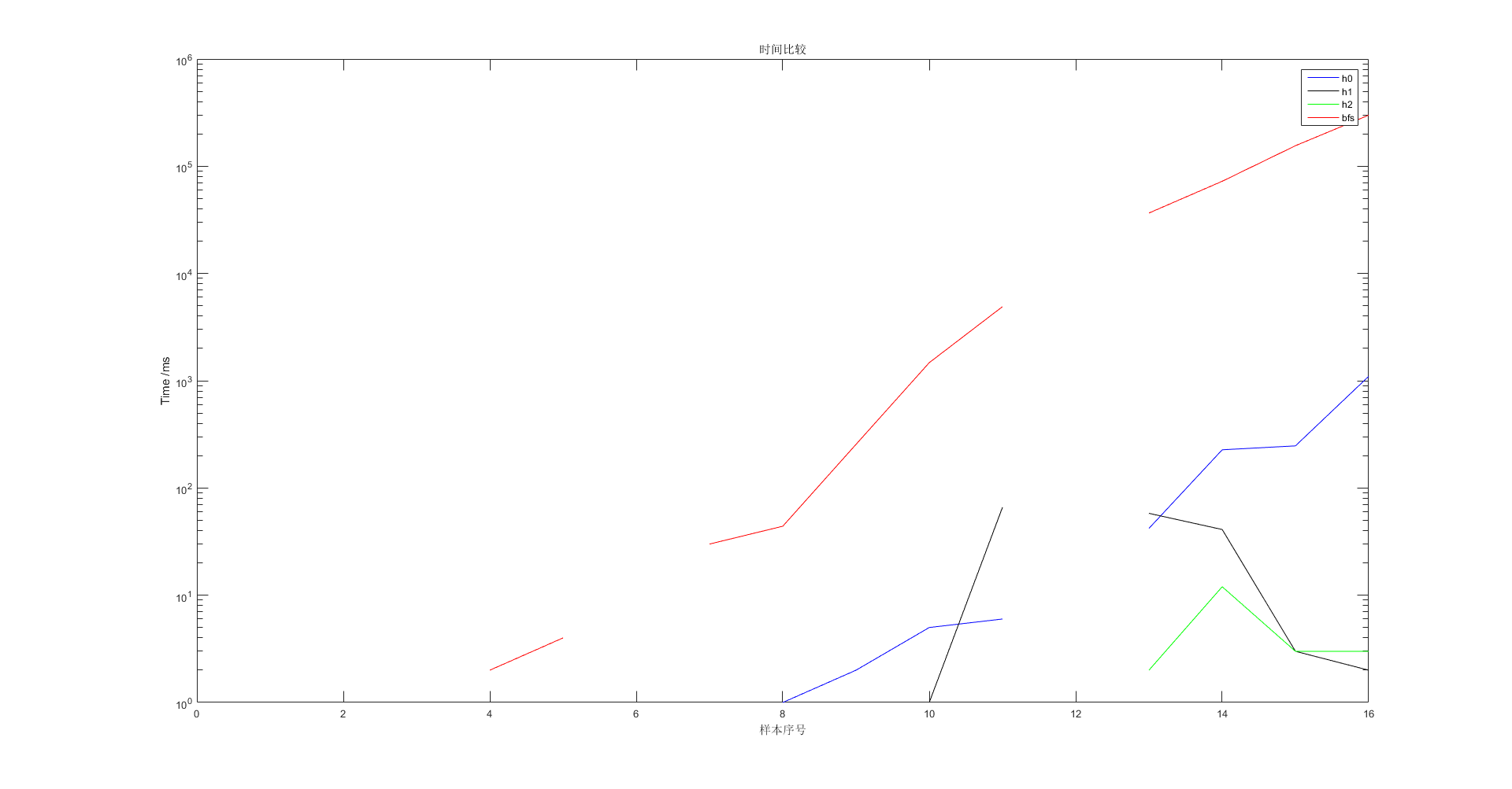
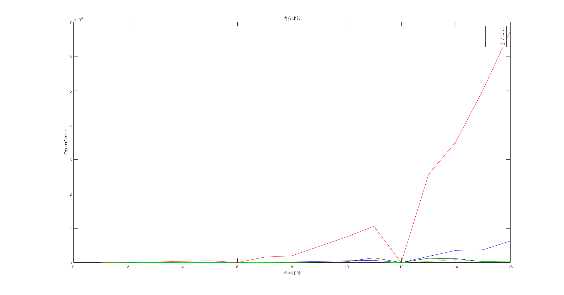
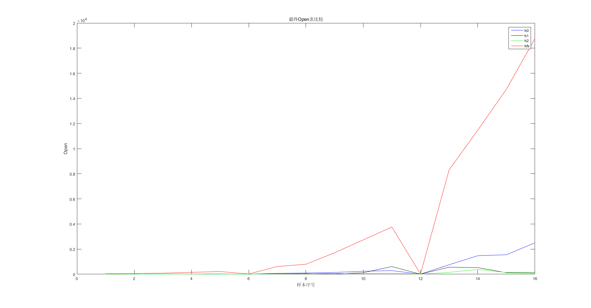
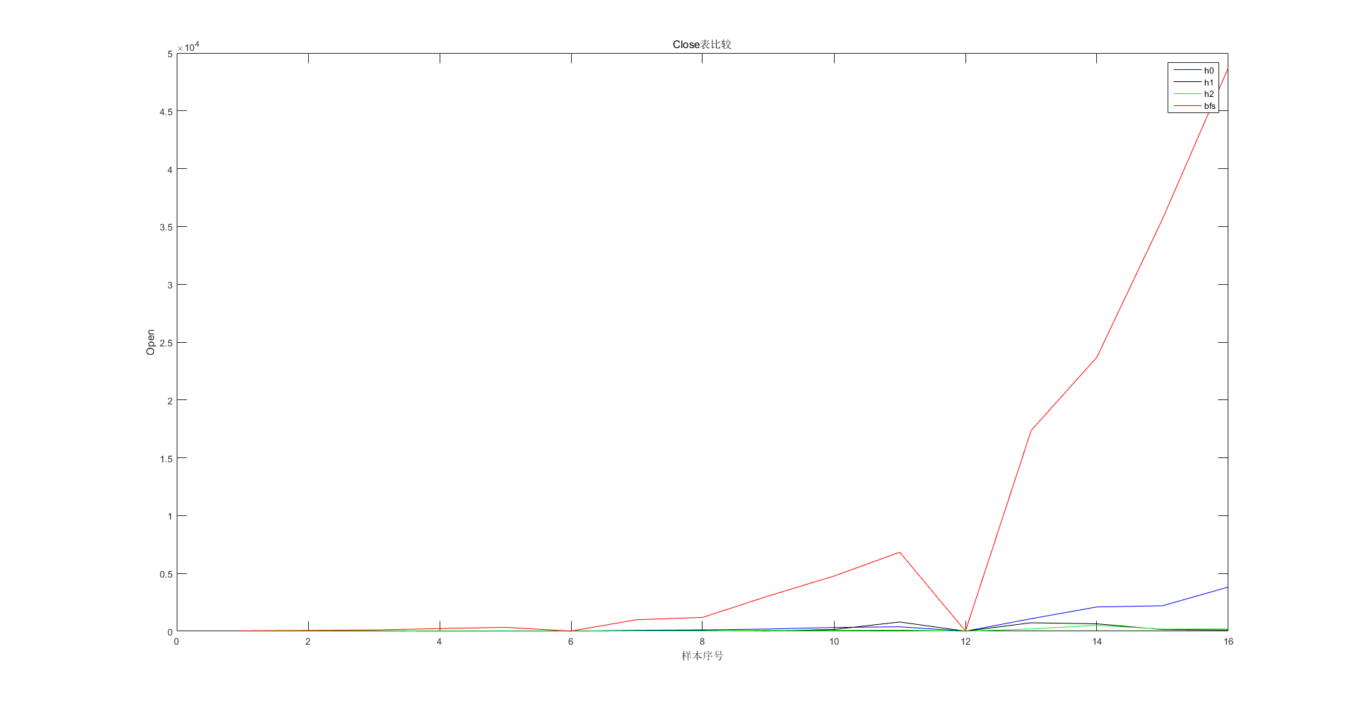
可以看到四种H评估函数都基本能得到最优解。
但是在时间上,二维曼哈顿和一维曼哈顿表现比较好。
空间上,同样是二维曼哈顿和一维曼哈顿表现较好。
BFS时间和空间都随着深度而近似指数增加,效率太低。
三 其他
1
本报告相关内容将发表在我的博客上(不定期更新):
A-Algorithm-and-8-Puzzle-Problem
代码(不定时更新):https://github.com/Vast-Stars/Algorithm/tree/master/8digit
2
八数码相关的游戏:
拼图:

https://github.com/netcan/SlidePuzzle
华容道:
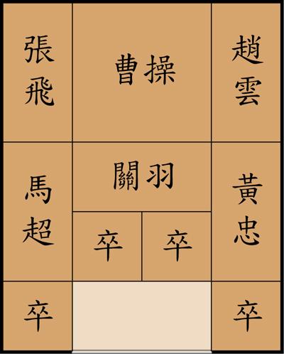
3
有个小问题:维基百科上的A*算法流程中,若子节点出现在Close表中,则不采取任何操作,这和书上更新F值相矛盾,为什么?
Reference
http://www.cnblogs.com/luxiaoxun/archive/2012/08/05/2624115.html
http://lucienwang.leanote.com/post/八数码——回顾BFS、双向广搜与A
https://www.cs.princeton.edu/courses/archive/fall12/cos226/assignments/8puzzle.html
http://www.cs.cmu.edu/afs/cs/Web/People/adamchik/15-121/labs/HW-7%20Slide%20Puzzle/lab.html
八数码最优解是否唯一判定
To be Updated……
k-nearest neighbors algorithm
代码在https://github.com/Vast-Stars/Algorithm/tree/master/KNN 上可以看到。 欢迎Star
一. 算法介绍
Main Idea:找出 $K$ 个距离未知样本$x$ 最近的已知样本点,以其中多数已知样本的类别作为$x$ 的类别。
需要考虑的问题:
- 算法优化。由于环境为Matlab,故无需考虑。
- 距离 的定义。根据特征空间性质定义距离,一般有以下几种:
- Euclidean Distance : $ d_{s,t}^2=(x_s-x_t)·(x_s-x_t)’ $ . 欧氏距离虽然很有用,但也有明显的缺点。 一:它将样品的不同特征之间的差别等同看待,这一点有时不能满足实际要求。 二:它没有考虑各特征的数量级(量纲),一般需要先对原始数据进行规范化处理再进行距离计算。
- Standardized Euclidean distance : $ d_{s,t}^2=(x_s-x_t)V ^ {-1} (x_s-x_t)’ $ where V is the n-by-n diagonal matrix whose $j$th diagonal element is ${S(j) }^2 $, where $S$ is the vector of standard deviations. 相比单纯的欧氏距离,标准欧氏距离能够有效的解决上述缺点。注意,这里的$V$在许多Matlab函数中是可以自己设定的,不一定非得取标准差,可以依据各变量的重要程度设置不同的值,如
knnsearch函数中的Scale属性。 - Mahalanobis distance : $ d_{s,t}^2=(x_s-x_t)C^{-1}(x_s-x_t)’ $ , C为协方差矩阵. 与欧式距离不同的是它考虑到各种特性之间的联系,并且是尺度无关的.如果协方差矩阵为单位矩阵,那么马氏距离就简化为欧式距离,如果协方差矩阵为对角阵,则其也可称为正规化的欧氏距离。缺点是:1 马氏距离的计算是建立在总体样本的基础上的,因为C是由总样本计算而来,所以马氏距离的计算是不稳定的;2 在计算马氏距离过程中,要求总体样本数大于样本的维数。3 协方差矩阵的逆矩阵可能不存在。
- Manhattan Distance :$D_{s,t}= \sum_{j=1}^n|x_{s_j}-x_{t_j}|$ . 曼哈顿距离是闵可夫斯基距离的一种特例(当$p=1$ 时)。
- Minkowski Distance : $D_{s,t}= \sqrt[p]{ \sum_{j=1}^n|x_{s_j}-x_{t_j} | ^p } $ . $p=1,2, \infty $ 时,闵可夫斯基距离分别等价于曼哈顿距离、欧氏距离、切比雪夫距离。闵可夫斯基距离由于是欧氏距离的推广,所以其缺点与欧氏距离大致相同。
- Chebychev Distance : $D_{s,t}= \max \limits_j |x_{s_j}-x_{t_j}|$
- Cosine Distance : $ D_{s,t}=1- \frac{x_s x_t’} { | x_s |_{2} | x_t | _{2} } $ 与Jaccard距离相比,Cosine距离不仅忽略0-0匹配,而且能够处理非二元向量,即考虑到变量值的大小。
- Correlation distance : $d_{s,t}=1- \frac{x_s x_t’} { \sqrt[]{ (x_s- \bar{x_s} )(x_t- \bar{x_t} )’}. \sqrt{ (x_t- \bar{x_t} ).(x_t- \bar{x_t} ) ‘ } } $ . Correlation距离主要用来度量两个向量的线性相关程度。
- Hamming Distance: $ d_{s,t}=( \frac{ \sharp (x_{s_j} \neq x_{t_j} ) } {n} )$ . 两个向量之间的汉明距离的定义为两个向量不同的变量个数所占变量总数的百分比。
- Jaccard Distance: $ d_{s,t}=( \frac{ \sharp [ (x_{s_j} \neq x_{t_j} ) \cap ( (x_{s_j} \neq 0) \cup(x_{t_j} \neq 0) ) ] } { \sharp (x_{s_j} \neq0) \cup(x_{t_j} \neq 0) } )$ . Jaccard距离常用来处理仅包含非对称的二元(0-1)属性的对象。很显然,Jaccard距离不关心0-0匹配,而Hamming距离关心0-0匹配。
- Spearman Distance: $d_{s,t}=1- \frac{ (r_s- \overline{r_s} )(r_t- \overline{r_t} )’} { \sqrt[]{ (r_s- \overline{r_s} ) (r_s- \overline{r_s} )’}. \sqrt{ (r_t- \overline{r_t} ) (r_t- \overline{r_t} )’} }$ .
KNN是一种lazy learning 算法,不需要预先训练,只需把所有训练数据载入内存,即可构成分类器。分类器也不含参数信息。
二. 实现
|
|
三. 测试
- $ X_{m \times n} $ : $m$ 个$n$ 维样本以行向量构成矩阵X ; $Y_{m \times 1}$ 对应储存着样本的类别信息(也可视作label)
- 统一采用十倍交叉验证 。
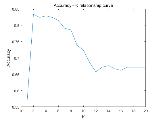
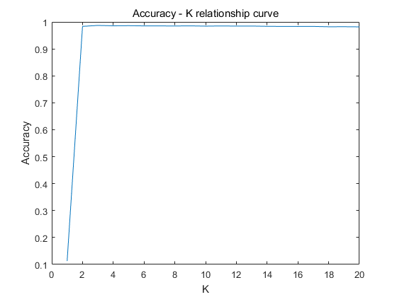
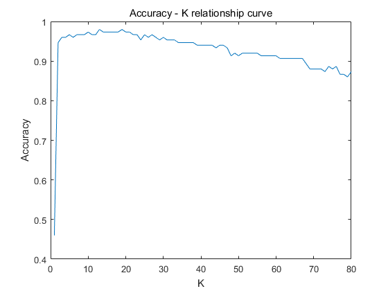
- 研究了K对准确率的影响。
1 SONAR
数据集全称: Connectionist Bench (Sonar, Mines vs. Rocks) Data Set
数据说明: 见UCI官网 )
本地文件名: SONAR.csv
运行结果:
|
|
2 USPS
数据集全称: Optical Recognition of Handwritten Digits Data Set
数据集来源: https://archive.ics.uci.edu/ml/machine-learning-databases/optdigits/optdigits.tes
https://archive.ics.uci.edu/ml/machine-learning-databases/optdigits/optdigits.tra
数据说明: 见UCI官网
本地文件名: optdigits.tes optdigits.tra
运行结果:
|
|
3 IRIS
数据集全称:Iris Data Set
数据集来源: https://archive.ics.uci.edu/ml/machine-learning-databases/iris/bezdekIris.data
数据说明: 见UCI官网
本地文件名: bezdekIris.data
运行结果:
|
|
最大准确率下K的取值波动较大。
四. 其他
1. K的取值
K的取值不宜过大。 最合适的K取值应该和类间距离有关。如果多类样本虽然线性可分,但是类与类距离较近的话,K只能取较小值。 反之,如果类间距离、类内距离都比较大,则KNN算法不易出错。
2. 插值,平滑曲线
KNN算法还可以用来做平滑曲线用,这个用法比较另类。比较适用于非连续曲线插值。
3. 寻找K个最短距离点的算法优化
一般来说,小规模问题都是用搜索的方法完成,例如用Dist=norm(X-repmat(x,size(X,1),1) );
大规模问题上,可以考虑GeoHash 、k-dimension tree、最大堆等算法。限于时间和篇幅,本文不予介绍。
Reference
Fisher Linear Discriminant Analysis (Fisher准则)
所有代码可以在 https://github.com/Vast-Stars/Algorithm/tree/master/Fisher 中看到。欢迎star
一. 算法介绍
这是Fisher在1936年提出的线性分类方法。对于二分类问题,训练集$D={ (\mathbf{x}_i,y_i),i=1,2\ldots n}$, 其中
${\mathbf{x}_i\in \mathscr{R^d}, y_i\in \lbrace 0,1\rbrace}$, 我们需要寻找一个权重向量$\mathbf{\omega}$ 和$\mathbf{\omega_0}$ 满足
Fisher准则的思路是将d维空间中的点$\mathbf{x_i}$投影到一条直线(分类超平面的法线)上,通过适当地选择直线的方向$\mathbf{\omega}$,有可能找到能够最大限度地区分各类样本数据点的投影方向。选择直线方向的思路是:最大化投影后类间距离和类内距离比(希望样本点向所求直线投影后,不同类别之间的距离大,相同类别之间的距离小)
其中$\mathbf{m}_i$ 表示第$i$ 类的均值。$\mathbf{S}_w$ 为类内散度矩阵(within-class scatter matrix),$\mathbf{S}_b$ 为类内散度矩阵(between-class scatter matrix)
其中$\Sigma_i$ 表示第$i$类的协方差矩阵。显然$\mathbf{S}_w$ 和$\mathbf{S}_b$ 均为对称矩阵
寻找$\mathbf{\omega}$使 $ J_F(\mathbf{\omega} )$ 最大,我们可以通过对$ J_F(\mathbf{\omega} )$ 求$\mathbf{\omega}$的偏导数并令其为$0$ 计算$\mathbf{\omega}$.
注意 ${ (\mathbf{m_0}-\mathbf{m_1} )}^T\mathbf{\omega}$ 和 $\mathbf{\omega}^T\mathbf{S}_{\mathbf{w} }\mathbf{\omega}$ 均为标量,且 $\frac{\partial(\mathbf{\omega}^T\mathbf{S}\mathbf{\omega} )}{\partial \mathbf{\omega} }=(\mathbf{S}+\mathbf{S}^T)\mathbf{\omega} $ .
同时,由于$\frac{ { (\mathbf{m_0}-\mathbf{m_1} )}^T\mathbf{\omega} }{\mathbf{\omega}^T\mathbf{S}_{\mathbf{w} }\mathbf{\omega} }$ 为标量, 因此
其中$\lambda\in \mathscr{R}$ ,由于我们在做线性分类时,主要关心直线的方向,因此可取$\lambda=1 $,如果$\mathbf{S}_w $ 可逆(如果不可逆,则用伪逆),则
关于 $\omega_0$ 的选择,有以下几种常见方法:
- 我们知道当投影直线的方向确定后,d维空间中的点$\mathbf{x}_i$ 在直线的投影位置确定。为此,我们希望$y=0$ 类的样本点到$0$ 的距离与$y=1$ 类的样本点到$0$ 的距离越接近越好(当一条直线上两个点之间的距离确定,两点构成线段的中垂面为最好的分类超平面)。于是 $ -\sum_{y=0}(\mathbf{\omega^T}\mathbf{x}+\omega_0)=\sum_{y=1}(\mathbf{\omega^T}\mathbf{x}+\omega_0) $ 。再设$ n_0、n_1 $ 分别为两类样本数量,因此:
- $\omega_0=-\frac{1}{2}(m_1+m_2)^T (S_\omega)^{-1}(m_1-m_2)-ln \frac{P(\omega_2)}{P(\omega_1)} $
- 暂无。待补充。
二. 测试
为了便于计算,统一规定如下:
- $X_{m\times n}$ $m$ 个$n$ 维样本以行向量构成矩阵X ; $Y_{m\times 1}$ 对应储存着样本的类别信息(也可视作label)
- 函数及关键语句附带说明。
- 注明数据来源。
- 统一采用十倍交叉验证 。
- F1=P*R/2(P+R)
1 SONAR
数据集全称: Connectionist Bench (Sonar, Mines vs. Rocks) Data Set
数据说明: 见UCI官网)
本地文件名: SONAR.csv
运行结果:
|
|
由于算法具有随机性,每次运行会有小范围波动。
2 USPS (3 && 8)
数据集全称: Optical Recognition of Handwritten Digits Data Set
数据集来源: https://archive.ics.uci.edu/ml/machine-learning-databases/optdigits/optdigits.tes
https://archive.ics.uci.edu/ml/machine-learning-databases/optdigits/optdigits.tra
数据说明: 见UCI官网
本地文件名: optdigits.tes optdigits.tra
运行结果:
|
|
由于算法具有随机性,每次运行会有小范围波动。
3 IRIS (Iris-setosa && Iris-versicolor)
数据集全称:Iris Data Set
数据集来源: https://archive.ics.uci.edu/ml/machine-learning-databases/iris/bezdekIris.data
数据说明: 见UCI官网
本地文件名: bezdekIris.data
运行结果:
|
|
IRIS第一类和第二三类线性可分。Fisher收敛到正解。
Reference
http://blog.leanote.com/post/directfly/Linear-Classification-Fisher-s-criterion-线性分类-Fisher准则
Majority Element Problem
All Code in this essay can be found in https://github.com/Vast-Stars/Algorithm/tree/master/Majority
Basic Report
1. Description
Given an array of size n, find the majority element.
The majority element is the element that appears more than ⌊ n/2 ⌋ times.
2. Algorithm
We can use the nature of the problem:
appears more than
⌊ n/2 ⌋times.
which means we can delete both a and b if a≠b, and this will not change the Majority Element in the remaining part of the array.
Specifically, I use a counter to record the number of occurrences of the target. I initialize target to array[0] , and sequential scan the array sequentially to array[i]. The counter will increase by 1 if array[i]==target, or otherwise will decrease by 1. If counter==0 then pick up next number as new target and continue this process until the entire array is scanned or counter >SIZE/2(which means program find a Majority element clearly).
3. Source Codes
The main function is demonstrated below:
|
|
Time complexity: O(n) Space complexity: O(1)
This function is tested by LeetCode: 169.Majority Element successfully.
4. Recursive process
|
|
Further Thinking
1. Algorithm optimization
In fact, we can improve this algorithm in 2 ways.
Use hash . Although it takes O(n) time complexity and O(n) space complexity, hash map(or table) is much convenient to deal with similar problem related statistics.
On the basis of the original algorithm, I change variable
sizein end conditioncount <= size / 2. I find thattargetonly needs to be greater than half the length of the remaining array, rather than half the total length. On the implementation, only one additional variable is required to record the last index(i) oftarget == 0and usesize = total_size- i - 1instead ofsize = total_size.Tested in 15,000 examples(Randomly generated, see source code for details), I get the speed difference between the 2 algorithms:
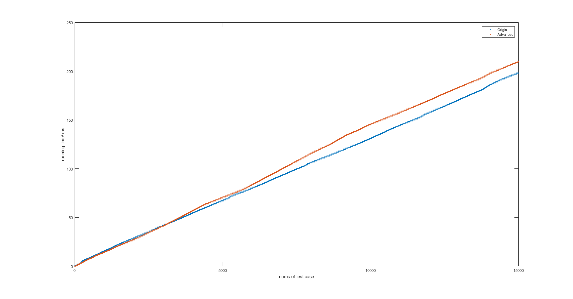
From the graph we can know it depends on the usage scenarios to choose and optimize algorithm to play its best performance.
2. Similar Problem Ⅰ: Find the Majority Element(appear greater or equal to⌊ n/2 ⌋ times )
To be honest, it’s confusing me for some time. I consider the cases of the parity of n, or whether there must be a solution to this problem . And it’s very difficult to generalize several cases of the algorithm together.
But later I came across another Majority problem(see blow), and I solved this problem effortlessly.
3. Similar Problem Ⅱ: Find the Majority Element(appear more than ⌊ n/3 ⌋ times )
Problem Source: LeetCode 229. Majority Element II
First of all, we can prove that there is up to 2 majority element . So it is natural to think about using 2 counters to record 2 targets(It seems to “doubled” previous algorithm). What’s differences is we need scan the entire array to count the number of target1 and target2 after the first traversal.
|
|
Time complexity: O(n) Space complexity: O(1)
This function is tested by LeetCode 229. Majority Element II successfully.